Direct archive access

The Direct Archive Access module lets you load data from any local or remote archive of CDF files directly into Speasy — no web service required.

This is useful when:

You have your own data files on disk or on a lab server
A public archive (e.g. CDAWeb) hosts files you want to access directly rather than through an API
You want to share a dataset configuration with colleagues

Once configured, the data appears in Speasy’s inventory and can be loaded with spz.get_data() like any other product.

How it works

Most space physics data archives follow a simple pattern: files are organized in folders by date (e.g. one CDF file per day, stored in yearly or monthly directories). Speasy exploits this predictable structure. You describe the URL pattern and file organization in a short YAML file, and Speasy handles the rest: it figures out which files to download for a given time range, loads them, and merges the results into a single SpeasyVariable.

Note

The data files must follow the ISTP CDF conventions. For non-ISTP files or other formats, see Custom file format support (advanced) below.

Quick start: adding a dataset

Step 1: Find the inventory directory

Create a YAML file (e.g. my_datasets.yaml) in Speasy’s user inventory directory. On Linux this is ~/.config/speasy/LPP/archive/, on macOS ~/Library/Application Support/speasy/LPP/archive/. You can confirm the exact path:

>>> import speasy as spz
>>> print(spz.data_providers.generic_archive.user_inventory_dir())

Step 2: Describe your dataset in YAML

Here is a minimal example for THEMIS-A FGM data hosted at CDPP, with one CDF file per day:

tha_fgm:
  inventory_path: my_data/THEMIS/THA
  master_cdf: http://cdpp.irap.omp.eu/themisdata/tha/l2/fgm/0000/tha_l2_fgm_00000000_v01.cdf
  split_frequency: daily
  split_rule: regular
  url_pattern: http://cdpp.irap.omp.eu/themisdata/tha/l2/fgm/{Y}/tha_l2_fgm_{Y}{M:02d}{D:02d}_v\d+.cdf
  use_file_list: true

Step 3: Restart Python and use it

After saving the YAML file, restart your Python session (the inventory is built at import time):

>>> import speasy as spz
>>> # Your dataset now appears in the inventory
>>> spz.inventories.data_tree.archive.my_data.THEMIS.THA.tha_fgm
>>> # Get data as usual
>>> tha_b = spz.get_data("archive/my_data/THEMIS/THA/tha_fgm/tha_fgl_btotal", "2018-06-01", "2018-06-02")

Tip

The individual variables within each dataset (like tha_fgl_btotal) are discovered automatically from the master CDF file. Use tab-completion in IPython/Jupyter to explore them.

YAML field reference

Field	Description
dataset_name (top-level key)	A name for your dataset. This becomes the last part of the inventory path.
inventory_path	Where the dataset appears in `spz.inventories.data_tree.archive`. Slashes create a nested hierarchy (e.g. `my_data/THEMIS/THA` → `archive.my_data.THEMIS.THA`).
master_cdf	URL or local path to a master CDF (or any sample CDF from this dataset). Speasy reads it once to discover which variables the dataset contains. Master CDFs are preferred because they are lightweight template files without actual data.
split_rule	How the files are organized: `regular` (predictable, one file per time period) or `random` (variable-length files like burst data). See Randomly split datasets (burst data).
split_frequency	Time granularity of the files: `daily`, `monthly`, `yearly`, or `none`. For `regular` datasets, this is how often a new file starts. For `random` datasets, this is how often a new folder starts (Speasy scans each folder for matching files).
url_pattern	The URL template for data files. Date placeholders are expanded for each time period. Can include Python regular expressions for unpredictable parts (e.g. file version numbers) when `use_file_list` is `true`. See the URL pattern placeholders table below.
use_file_list	If `true`, Speasy lists the files in each directory and selects the last one matching the URL pattern. Set this to `true` when parts of the filename are unpredictable (like version numbers). Default: `false`.
fname_regex	Only for `random` split datasets. A Python regular expression to extract the start date (and optionally stop date and version) from each filename. See Randomly split datasets (burst data).

URL pattern placeholders

The url_pattern uses Python str.format() syntax. Available placeholders:

Placeholder	Meaning	Example output
`{Y}`	4-digit year	`2018`
`{y}`	2-digit year	`18`
`{M}`	Month (no padding)	`1` .. `12`
`{M:02d}`	Month (zero-padded)	`01` .. `12`
`{D}`	Day (no padding)	`1` .. `31`
`{D:02d}`	Day (zero-padded)	`01` .. `31`
`{j}`	Day of year	`1` .. `366`
`{H}`	Hour (24h)	`0` .. `23`

Regex parts of the pattern (like \d+ for version numbers) are only interpreted when use_file_list: true.

Randomly split datasets (burst data)

Some datasets don’t produce one file per day. Instead, files cover irregular time intervals (e.g. burst-mode data that only records during events). For these, use split_rule: random.

The key difference is the fname_regex field: a regular expression that Speasy applies to each filename to extract the time range it covers.

mms1_fpi_brst_l2_des_moms:
  inventory_path: cda/MMS/MMS1/FPI/BURST/MOMS
  master_cdf: "https://cdaweb.gsfc.nasa.gov/pub/software/cdawlib/0MASTERS/mms1_fpi_brst_l2_des-moms_00000000_v01.cdf"
  split_rule: random
  split_frequency: monthly
  url_pattern: 'https://cdaweb.gsfc.nasa.gov/pub/data/mms/mms1/fpi/brst/l2/des-moms/{Y}/{M:02d}/mms1_fpi_brst_l2_des-moms_{Y}{M:02d}\d+_v\d+.\d+.\d+.cdf'
  use_file_list: true
  fname_regex: 'mms1_fpi_brst_l2_des-moms_(?P<start>\d+)_v(?P<version>[\d\.]+)\.cdf'

How it works: for each month in the requested time range, Speasy lists all files in the folder, applies fname_regex to extract the start time from each filename, keeps only the files that overlap with the requested interval, and loads them.

fname_regex named groups:

(?P<start>...) — start date extracted from the filename (mandatory). Must be parsable as a date.
(?P<stop>...) — stop date (optional). If absent, Speasy assumes each file ends when the next one starts.
(?P<version>...) — file version (optional). Used to pick the latest version when multiple exist.

Extra inventory directories

Beyond the default user directory, you can tell Speasy to scan additional directories for YAML files:

[ARCHIVE]
extra_inventory_lookup_dirs = /shared/lab/speasy_inventories,/another/path

Or via the environment variable SPEASY_ARCHIVE_EXTRA_INVENTORY_LOOKUP_DIRS.

Custom file format support (advanced)

If your data files are not ISTP-compliant CDF files, you can write a custom reader function and use speasy.core.direct_archive_downloader.get_product directly.

Your reader function receives a file URL and a variable name, and returns a SpeasyVariable (or None):

from speasy.products import SpeasyVariable

def my_reader(url: str, variable: str, **kwargs) -> SpeasyVariable or None:
    # Load data from url, build and return a SpeasyVariable
    ...

Then call get_product with your reader:

from speasy.core.direct_archive_downloader import get_product

data = get_product(
    url_pattern="https://example.com/data/{Y}/{M:02d}/mydata_{Y}{M:02d}{D:02d}_v\d+.cdf",
    start_time="2023-06-19",
    stop_time="2023-06-20",
    variable="B",
    split_rule="regular",
    split_frequency="daily",
    use_file_list=True,
    file_reader=my_reader,
)

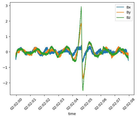
Example: reading non-ISTP Solar Orbiter LFR snapshots

This example shows a custom reader for Solar Orbiter RPW/LFR waveform snapshots. These files contain multiple snapshots at different sampling rates packed into a single CDF, so the standard reader cannot handle them.

import speasy as spz
from speasy.products import SpeasyVariable, VariableTimeAxis, DataContainer
from speasy.core.direct_archive_downloader import get_product
from speasy.core.any_files import any_loc_open
import numpy as np
import pycdfpp
import matplotlib.pyplot as plt

def snapshots_B_custom_reader(url, variable='B', sampling = 24576.):
    cdf=pycdfpp.load(any_loc_open(url,cache_remote_files=True).read())
    # all snapshots for different sampling rates are stored in the same variable
    # so we need to build an index of the snapshots with the desired sampling rate
    indexes = cdf["SAMPLING_RATE"].values[:] == sampling
    # build time axis from each snapshot start time and sampling rate
    star_times = pycdfpp.to_datetime64(cdf["Epoch"].values[indexes]).astype(np.int64)
    time = np.linspace(star_times, star_times+2048*int(1e9/sampling),num=2048).astype('datetime64[ns]').T.reshape(-1)
    sel_values = cdf[variable].values[indexes]
    values = np.empty((sel_values.shape[0]*sel_values.shape[2],3), sel_values.dtype)
    values[:,0] = sel_values[:,0,:].reshape(-1)
    values[:,1] = sel_values[:,1,:].reshape(-1)
    values[:,2] = sel_values[:,2,:].reshape(-1)
    if 'RTN' in variable:
        labels = ['Bxrtn', 'Byrtn', 'Bzrtn']
    else:
        labels = ['Bx', 'By', 'Bz']
    return SpeasyVariable(axes=[VariableTimeAxis(values= time)],values=DataContainer(values), columns=labels)


lfr_b_F2 = get_product(url_pattern="http://sciqlop.lpp.polytechnique.fr/cdaweb-data/pub/data/solar-orbiter/rpw/science/l2/lfr-surv-swf-b/{Y}/solo_l2_rpw-lfr-surv-swf-b_{Y}{M:02}{D:02}_v\d+.cdf",
                    start_time="2023-06-19T02:01:59",
                    stop_time="2023-06-19T02:02:08",
                    variable="B",
                    split_rule="regular",
                    split_frequency="daily",
                    use_file_list=True,
                    file_reader=snapshots_B_custom_reader,
                    sampling = 256.
                    )
plt.figure()
lfr_b_F2.plot()
plt.show()

This produces the following plot: